Carbon accounting can be time-consuming, especially when done manually. While Avarni simplifies this process, we know many still rely on spreadsheets. This article offers guidance, and you can also explore our comprehensive list of global emission factor databases to find the data you need in one place.
One of the most time-consuming categories to baseline under the GHG Protocol is Scope 3 Category 1: Purchased Goods and Services. Unfortunately, it’s also often the largest source of emissions, making accuracy especially important.
Starting with the spend-based method is a practical first step. It allows an initial baseline to be established across the entire category, with more accurate activity-based calculations applied later to the most material areas.
Even so, anyone who has completed a spend-based inventory for Category 1 emissions will recognise the challenge: clarifying spend categories, dealing with messy or inconsistent data, and manually mapping emission factors. There are strategies that can be applied in spreadsheets to make this process easier and reduce the risk of errors — let’s dig into them.
Choosing the right factor database
The choice of emission factor database will depend on the level of detail required. The EPA database includes a detailed list of more than 1,000 spend categories, allowing for relatively accurate estimates from the outset — provided the relevant categories are well understood. By comparison, EXIOBASE offers around 180 more generalised categories, which are easier to apply but typically result in less precise estimates.
There are more considerations that should affect your choice of database (see our article on choosing an emission factor database), but the number of categories of spend in the database will be the single most impactful thing that affects how much time you spend on the next steps, and how accurate your final inventory is. More categories = more time spent = more detail.
Choosing a primary category column to match against
This is the second most important thing that will affect the accuracy and time spent building the inventory. You have to choose an appropriate column in your spend data that represents the products purchased most accurately. There may be multiple levels of categorisation with greater and greater detail. Choose which level of detail is most appropriate for your case — often the “Account” or “Account Name” field is a good candidate.
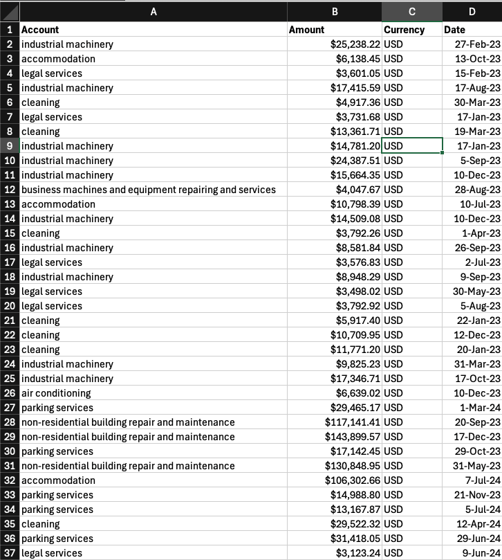
How straightforward this step is will depend on the quality of the available spend data. In many cases, some level of spend categorisation will be sufficient for mapping emission factors. However, if the data consists of inconsistent or highly fragmented categories with hundreds of variations, the process becomes significantly more complex.
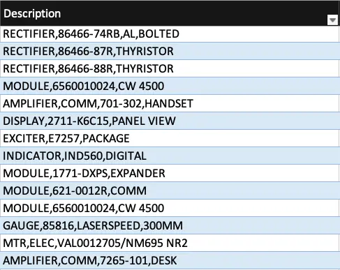
Avoid relying on free-text description fields to match emission factors when a higher-level, structured categorisation is available. While matching on descriptions can produce a more granular inventory, it is time-consuming and makes it much harder to produce clear, consistent reporting once the inventory is complete. Using clean, standardised categories results in a process that is both more efficient and easier to interpret.
Matching emission factors to the primary categories
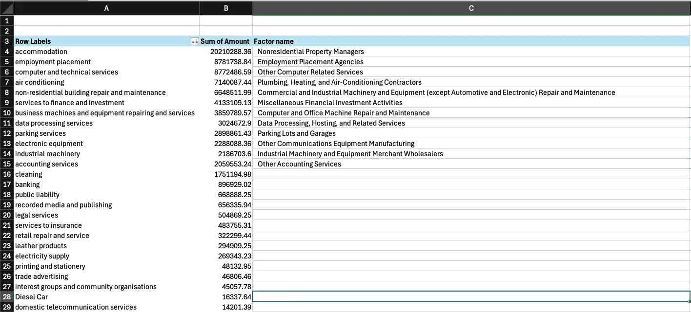
Create a pivot table based on the column that you choose as the primary category. Then, order your categories from highest spend to lowest, and work through each row to choose the most appropriate emission factor. This is really boring, so you want to start with your most material categories because by the time you get to the end your matching will be more careless because of how tired it’ll make your brain!
Search for an appropriate factor by looking for keywords in factor names that match keywords in the primary category, such as “beverages” or “legal”. If there’s no factor available, try searching using a keyword that relates to the higher level category that the primary category is in. Eg. If you’re looking for a “consulting” factor and none is available, try searching for “services”. Or if you’re searching for “oranges” and nothing comes up, try “fruit”, and then “crops”. Some databases will have catch-all factors for different activities that have the keywords “all other” in them, this is good to search for if you run out of options.
The most popular databases, such as EPA, DEFRA and EXIOBASE, will have enough breadth and depth to cover any purchase that a business could make.
Drilling down into material categories
Once you’ve completed the first level of mappings, the job could be done, depending on the level of detail you're looking for. In many cases, it’s worth going to sub-categories for the most material primary categories that constitute the largest spend, particularly if the primary category is very general, such as “Food”. A good rule of thumb is to drill into the categories that make up an aggregate 80% of the total spend — note that this will be a minority of the total number of categories, since the majority of spend will be skewed to a few categories.
To drill into these, add the second categorisation to the original pivot table, and match factors to the sub-categories for the group of primary categories that constitute 80% of the spend.
Matching factors based on supplier industries
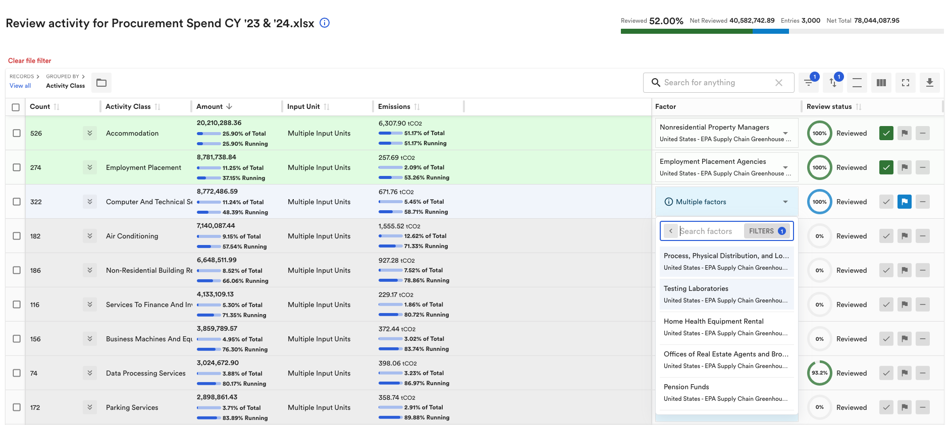
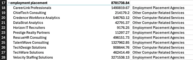
In cases where more material primary categories are very general, such as “Services”, and you don’t have a sub-category to refer to — you can match emission factors on a supplier-specific basis instead.
Create a pivot table with the first level categorisation and then the supplier name under that, have a tab open in Google, and search the supplier name to find out what industry they operate in, and what kind of products they produce. Use this information to choose the most appropriate emission factor to apply to that supplier. Below, we’ve differentiated between tech services and recruitment services under the same high level “employment placement” category.
Ensuring consistency for future datasets
Once you’ve done all this work, you will want to save the emission factor mappings you have done on a seperate sheet for future reference, to ensure you can build a consistent methodology year-on-year, and not double up on the same work that you did this year. Maintaining the same methodology will be important to make sure that any changes in emissions once activity based calculations are applied are not a result of a change in mapping methodology.
Summary
Building a spend-based emissions calculation for Scope 3 is a process of dividing and conquering:
- Choose a factor database to use depending on your needs. The more detailed the factor categories, the more time it will take to build the inventory.
- Choose a primary column that categorises the spend data based on type of good or service purchased, and match the entire dataset to the emission factors based on the categories in this column. Do not match to a free text description field with lots of unique values to avoid a time black hole and messy reporting later on.
- Split off the categories that make up the top 80% of spend, and “drill-down” into these categories to a second level of more detailed categorisations, if available. Match emissions factors to these more detailed categories, so that you have a more accurate view of the most material categories of emissions.
- If a second level category is not available, or if otherwise needed, match emission factors to the most material suppliers based on the industry they sit in.
- Document matching logic for each step in a seperate sheet for future reference, to ensure consistency in methodology year on year for the same inventory.
Scale spend-based Scope 3 calculations
Want to automate the accurate matching of emission factors to your data, and ensure consistency year on year without having to track it yourself? With Avarni, you can:
- Automate the mapping of emission factors to your data using AI from a range of the most popular spend-based factor databases used in corporate inventories, such as EPA, DEFRA and EXIOBASE — eliminating risk of using a factor that may not be the most appropriate.
- Upload your own emission factor database to match to if it’s not already available on Avarni.
- Review the results in a specialised workflow designed for top-level review of the mappings, followed by drilling-down, ensuring you put your focus on the most material categories first.
- One-click search of supplier names on Google, so you can quickly check their industry.
- Auto-saving of factor mappings as you review, ensuring you get the same results when you upload data next year.
Contact us to learn more.